
Metal vs. Non-Metal Classification on matbench_expt_is_metal#
Using Metallicity Features + XGBoost + Threshold Tuning#
![]()
This script demonstrates how to:
Load the matbench_expt_is_metal dataset.
Parse each composition to extract newly added “metallic” features (via the SMACT-based module code provided).
Build a pipeline to train an XGBoost classifier on these features.
Tune XGBoost hyperparameters and the ‘metallicity_threshold’ parameter to see how it affects classification performance.
Evaluate via cross-validation, confusion matrices, classification metrics.
Perform SHAP feature analysis to understand feature importance.
# Install the required packages
try:
    import google.colab

    IN_COLAB = True
except:
    IN_COLAB = False

if IN_COLAB:
    !uv pip install smact[ml] --quiet
import warnings

warnings.filterwarnings("ignore")

import numpy as np
import pandas as pd

# Machine learning / model-related imports
from sklearn.model_selection import StratifiedKFold, GridSearchCV, train_test_split
from sklearn.metrics import accuracy_score, classification_report, confusion_matrix
from xgboost import XGBClassifier

# SHAP + matplotlib + seaborn for plotting and feature importance analysis
import shap
import matplotlib.pyplot as plt
import seaborn as sns

# composition parsing and new features
from pymatgen.core import Composition
1. Loading the full matbench_expt_is_metal dataset#
try:
    from matminer.datasets import load_dataset

    # Load the full dataset from matminer
    df = load_dataset("matbench_expt_is_metal")
    # The dataframe should have columns: ["composition", "is_metal"]
    # Confirm we have 4921 entries
    print(f"Loaded dataset with {len(df)} entries.")

except ImportError:
    raise ImportError("Please install matminer or load the CSV file version of the dataset.")
Loaded dataset with 4921 entries.
2. Feature extraction - Intermetallic descriptors#
def extract_metallicity_features(comp_str: str) -> dict:
    """
    Given a composition string, parse it and return
    a dictionary of the new metallicity features.
    """
    # Convert string to Composition
    comp = Composition(comp_str)

    # Compute features using the newly introduced SMACT functions
    from smact.metallicity import (
        get_metal_fraction,
        get_d_block_element_fraction,
        get_distinct_metal_count,
        get_pauling_test_mismatch,
        metallicity_score,
    )

    feats = {}
    feats["metal_fraction"] = get_metal_fraction(comp)
    feats["d_block_element_fraction"] = get_d_block_element_fraction(comp)
    feats["distinct_metal_count"] = get_distinct_metal_count(comp)
    feats["pauling_mismatch"] = get_pauling_test_mismatch(comp)
    feats["metallicity_score"] = metallicity_score(comp)

    return feats


print("Extracting metallicity features for each sample ...")
all_features = []
for i, row in df.iterrows():
    feats = extract_metallicity_features(row["composition"])
    all_features.append(feats)

X_featurized = pd.DataFrame(all_features)
y = df["is_metal"].values

print("Feature extraction complete!")
print(X_featurized.head())
Extracting metallicity features for each sample ...
Feature extraction complete!
   metal_fraction  d_block_element_fraction  distinct_metal_count  \
0        0.600000                  0.600000                     2
1        0.333333                  0.333333                     2
2        0.448276                  0.068966                     3
3        0.448276                  0.068966                     3
4        0.500000                  0.500000                     1

   pauling_mismatch  metallicity_score
0          0.433333           0.692917
1          0.840000           0.537464
2          0.403333           0.582851
3          0.388333           0.583601
4          0.686667           0.582333
3. Model + Cross-validation + Threshold tuning#
def custom_threshold_predictions(proba, threshold):
    """
    Convert continuous probabilities to binary predictions using a custom threshold.
    By default, the classifier uses 0.5. We allow a different cutoff to see how
    sensitive the classification is to the intermetallic threshold logic.
    """
    return (proba >= threshold).astype(int)


# We will set up a grid of XGBoost hyperparameters + thresholds to tune:
param_grid = {
    "learning_rate": [0.01, 0.1],
    "max_depth": [3, 6],
    "n_estimators": [100, 200],
    # We'll handle the metallicity_threshold external to XGB's own param_grid
    # so we won't put threshold here. We'll do a loop over thresholds.
}
4. Hyperparameter/Threshold search with cross-validation#
cv = StratifiedKFold(n_splits=5, shuffle=True, random_state=42)

best_score = -np.inf
best_params = {}
thresholds = [0.5, 0.6, 0.7, 0.8]  # metallicity_threshold

for lr in param_grid["learning_rate"]:
    for md in param_grid["max_depth"]:
        for ne in param_grid["n_estimators"]:
            for thres in thresholds:
                # Initialize the classifier
                clf = XGBClassifier(
                    learning_rate=lr,
                    max_depth=md,
                    n_estimators=ne,
                    use_label_encoder=False,
                    eval_metric="logloss",
                    random_state=42,
                )

                # We'll do manual cross-val:
                fold_accuracies = []
                for train_idx, val_idx in cv.split(X_featurized, y):
                    X_train_cv = X_featurized.iloc[train_idx]
                    y_train_cv = y[train_idx]
                    X_val_cv = X_featurized.iloc[val_idx]
                    y_val_cv = y[val_idx]

                    # Train
                    clf.fit(X_train_cv, y_train_cv)

                    # Predict with custom threshold
                    y_proba_val = clf.predict_proba(X_val_cv)[:, 1]
                    y_pred_val = custom_threshold_predictions(y_proba_val, thres)

                    fold_accuracies.append(accuracy_score(y_val_cv, y_pred_val))

                mean_acc = np.mean(fold_accuracies)

                # Track best
                if mean_acc > best_score:
                    best_score = mean_acc
                    best_params = {
                        "learning_rate": lr,
                        "max_depth": md,
                        "n_estimators": ne,
                        "threshold": thres,
                        "cv_accuracy": best_score,
                    }

print("Best parameters found:")
print(best_params)

# this is still pending a cv of the metallicity scores model weighting
Best parameters found:
{'learning_rate': 0.1, 'max_depth': 6, 'n_estimators': 200, 'threshold': 0.5, 'cv_accuracy': 0.8575496265114936}
5. Retrain best model on full training set & evaluate#
# Usually you'd do a train/test split. Let's do that for a final check:
X_train, X_test, y_train, y_test = train_test_split(X_featurized, y, test_size=0.2, random_state=42, stratify=y)
best_model = XGBClassifier(
learning_rate=best_params["learning_rate"],
max_depth=best_params["max_depth"],
n_estimators=best_params["n_estimators"],
use_label_encoder=False,
eval_metric="logloss",
random_state=42,
)
best_model.fit(X_train, y_train)
# Evaluate on test set
y_proba_test = best_model.predict_proba(X_test)[:, 1]
y_pred_test = custom_threshold_predictions(y_proba_test, best_params["threshold"])
test_acc = accuracy_score(y_test, y_pred_test)
print(f"\nTest Accuracy: {test_acc:.3f} with threshold={best_params['threshold']}")
print("\nClassification Report:")
print(classification_report(y_test, y_pred_test))
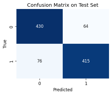
cm = confusion_matrix(y_test, y_pred_test)
plt.figure(figsize=(4, 3), dpi=120)
sns.heatmap(cm, annot=True, cmap="Blues", fmt="d", cbar=False)
plt.title("Confusion Matrix on Test Set")
plt.xlabel("Predicted")
plt.ylabel("True")
plt.show()
Test Accuracy: 0.858 with threshold=0.5

Classification Report:
              precision    recall  f1-score   support

       False       0.85      0.87      0.86       494
        True       0.87      0.85      0.86       491

    accuracy                           0.86       985
   macro avg       0.86      0.86      0.86       985
weighted avg       0.86      0.86      0.86       985
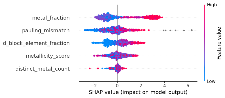
6. SHAP feature analysis#
print("\nPerforming SHAP analysis...")
# Create an explainer with the best model
explainer = shap.TreeExplainer(best_model)
shap_values = explainer.shap_values(X_test)
# Summary plot
shap.summary_plot(shap_values, features=X_test, feature_names=X_test.columns)
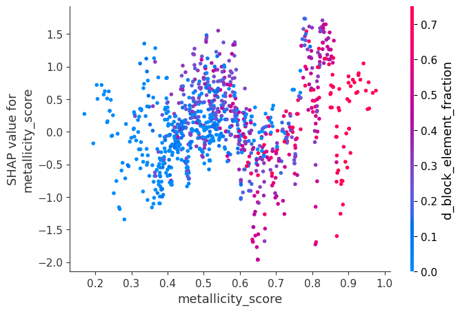
# Dependence plot example (for any feature, say 'metallicity_score')
if "metallicity_score" in X_test.columns:
shap.dependence_plot("metallicity_score", shap_values, X_test, display_features=X_test)
print("\nAll done!")
Performing SHAP analysis...
All done!