Exploring crystal space#
Our goal is to generate, analyze, and categorize chemical compositions, making it easier to discover interesting and useful materials. This tutorial is based on a publication in Faraday Discussions.
1. Getting started#
In this tutorial, we’ll:
Generate binary chemical compositions using the SMACT filter.
Explore whether these compositions exist in the Materials Project database.
Categorize the compositions based on whether they pass the SMACT filter and whether they are found in the database.
The final phase will categorize the compositions into four distinct categories based on their properties. The categorization is based on whether a composition is allowed by the SMACT filter (smact_allowed) and whether it is present in the Materials Project database (mp). The categories are as follows:
smact_allowed |
mp |
label |
|---|---|---|
yes |
yes |
standard |
yes |
no |
missing |
no |
yes |
interesting |
no |
no |
unlikely |
2. Generating compositions#
First, we’ll create binary chemical compositions using the SMACT filter. The SMACT filter is a smart tool that helps us select compositions based on important chemical rules, such as oxidation states and electronegativity.
To generate these compositions, we’ll use a function called generate_composition_with_smact. This function allows us to enumerate all possible binary compositions and filter them based on the SMACT rules.
Key parameters:#
num_elements: Number of elements in the composition (e.g., 2 for binary).max_stoich: The maximum ratio of each element (e.g., 8 could mean up to 8 atoms of each element).max_atomic_num: Maximum atomic number for the elements considerednum_processes: Number of processes to run in parallel to speed up calculations.save_path: Where to save the generated compositions.
![]()
# Install the required packages
try:
    import google.colab

    IN_COLAB = True
except:
    IN_COLAB = False

if IN_COLAB:
    !uv pip install smact[crystal_space] --quiet
from smact.utils.crystal_space.generate_composition_with_smact import (
    generate_composition_with_smact,
)
df_smact = generate_composition_with_smact(
    num_elements=2,
    max_stoich=8,
    max_atomic_num=103,
    num_processes=8,
    save_path="data/binary/df_binary_label.pkl",
    oxidation_states_set="smact14",
)
#1. Generating all possible combinations of elements...
Number of generated combinations: 5253
#2. Generating all possible stoichiometric combinations...
100%|██████████| 5253/5253 [00:05<00:00, 923.16it/s]
Number of generated compounds: 336192
Number of generated compounds (unique): 225879
#3. Filtering compounds with SMACT...
100%|██████████| 4656/4656 [00:02<00:00, 1856.51it/s]
#4. Making data frame of results...
Number of compounds allowed by SMACT: 13464
Saved to data/binary/df_binary_label.pkl
df_smact
| smact_allowed | |
|---|---|
| Cr4C5 | True |
| Bk3Bi8 | False |
| Cf6F5 | False |
| Hf5Pb4 | False |
| CeHg2 | False |
| ... | ... |
| Be4Xe3 | False |
| NpSb5 | False |
| Mn4Al | False |
| Th6Ti7 | False |
| H7Rn | False |
225879 rows × 1 columns
3. Download data from the Materials Project#
Next, we download data from the Materials Project api using the download_mp_data function. This function allows us to download data for a given number of elements and maximum stoichiometry. The data includes the chemical formula, energy, and other properties of the compounds.
download_mp_data function takes in the following parameters:
Key parameters:#
mp_api_key: your Materials Project API keynum_elements: Number of elements in the composition (e.g., 2 for binary).max_stoich: The maximum ratio of each element (e.g., 8 could mean up to 8 atoms of each element).save_dir: Where to save the downloaded data
mp_api_key = "" # Add your Materials Project API key here
save_mp_dir = "data/binary/mp_data"
from smact.utils.crystal_space.download_compounds_with_mp_api import download_mp_data

# download data from MP for binary compounds
docs = download_mp_data(
    mp_api_key=mp_api_key,
    num_elements=2,
    max_stoich=8,
    save_dir=save_mp_dir,
)
0%| | 0/22 [00:00<?, ?it/s]
Downloading data for A2B3...
Retrieving SummaryDoc documents: 100%|██████████| 1190/1190 [00:01<00:00, 854.30it/s]
  5%|▍         | 1/22 [00:11<03:52, 11.07s/it]
Downloading data for A2B5...
Retrieving SummaryDoc documents: 100%|██████████| 308/308 [00:00<00:00, 1256659.18it/s]
  9%|▉         | 2/22 [00:14<02:15,  6.79s/it]
Downloading data for A2B7...
Retrieving SummaryDoc documents: 100%|██████████| 98/98 [00:00<00:00, 403377.62it/s]
 14%|█▎        | 3/22 [00:17<01:32,  4.84s/it]
Downloading data for A3B4...
Retrieving SummaryDoc documents: 100%|██████████| 616/616 [00:00<00:00, 2350947.46it/s]
 18%|█▊        | 4/22 [00:21<01:24,  4.71s/it]
Downloading data for A3B5...
Retrieving SummaryDoc documents: 100%|██████████| 486/486 [00:00<00:00, 54624.75it/s]
 23%|██▎       | 5/22 [00:27<01:23,  4.93s/it]
Downloading data for A3B7...
Retrieving SummaryDoc documents: 100%|██████████| 132/132 [00:00<00:00, 527786.59it/s]
 27%|██▋       | 6/22 [00:30<01:09,  4.33s/it]
Downloading data for A3B8...
Retrieving SummaryDoc documents: 100%|██████████| 93/93 [00:00<00:00, 302849.59it/s]
 32%|███▏      | 7/22 [00:32<00:54,  3.63s/it]
Downloading data for A4B5...
Retrieving SummaryDoc documents: 100%|██████████| 175/175 [00:00<00:00, 1073104.09it/s]
 36%|███▋      | 8/22 [00:35<00:49,  3.52s/it]
Downloading data for A4B7...
Retrieving SummaryDoc documents: 100%|██████████| 151/151 [00:00<00:00, 642332.56it/s]
 41%|████      | 9/22 [00:39<00:45,  3.48s/it]
Downloading data for A5B6...
Retrieving SummaryDoc documents: 100%|██████████| 136/136 [00:00<00:00, 363559.81it/s]
 45%|████▌     | 10/22 [00:41<00:37,  3.12s/it]
Downloading data for A5B7...
Retrieving SummaryDoc documents: 100%|██████████| 31/31 [00:00<00:00, 70626.52it/s]
 50%|█████     | 11/22 [00:43<00:30,  2.81s/it]
Downloading data for A5B8...
Retrieving SummaryDoc documents: 100%|██████████| 71/71 [00:00<00:00, 300803.62it/s]
 55%|█████▍    | 12/22 [00:45<00:26,  2.60s/it]
Downloading data for A6B7...
Retrieving SummaryDoc documents: 100%|██████████| 43/43 [00:00<00:00, 282688.20it/s]
 59%|█████▉    | 13/22 [00:47<00:22,  2.45s/it]
Downloading data for A7B8...
Retrieving SummaryDoc documents: 100%|██████████| 30/30 [00:00<00:00, 89813.79it/s]
 64%|██████▎   | 14/22 [00:50<00:18,  2.37s/it]
Downloading data for AB...
Retrieving SummaryDoc documents: 100%|██████████| 3634/3634 [00:04<00:00, 895.90it/s]
 68%|██████▊   | 15/22 [01:03<00:39,  5.64s/it]
Downloading data for AB2...
Retrieving SummaryDoc documents: 100%|██████████| 4753/4753 [00:07<00:00, 644.81it/s]
 73%|███████▎  | 16/22 [01:21<00:55,  9.30s/it]
Downloading data for AB3...
Retrieving SummaryDoc documents: 100%|██████████| 5628/5628 [00:05<00:00, 1088.41it/s]
 77%|███████▋  | 17/22 [01:43<01:05, 13.12s/it]
Downloading data for AB4...
Retrieving SummaryDoc documents: 100%|██████████| 686/686 [00:00<00:00, 1829175.17it/s]
 82%|████████▏ | 18/22 [01:48<00:43, 10.78s/it]
Downloading data for AB5...
Retrieving SummaryDoc documents: 100%|██████████| 544/544 [00:00<00:00, 1890390.54it/s]
 86%|████████▋ | 19/22 [01:52<00:26,  8.74s/it]
Downloading data for AB6...
Retrieving SummaryDoc documents: 100%|██████████| 221/221 [00:00<00:00, 795657.67it/s]
 91%|█████████ | 20/22 [01:55<00:14,  7.04s/it]
Downloading data for AB7...
Retrieving SummaryDoc documents: 100%|██████████| 85/85 [00:00<00:00, 303676.18it/s]
 95%|█████████▌| 21/22 [01:57<00:05,  5.54s/it]
Downloading data for AB8...
Retrieving SummaryDoc documents: 100%|██████████| 37/37 [00:00<00:00, 125863.14it/s]
100%|██████████| 22/22 [01:59<00:00,  5.42s/it]
4. Categorise compositions#
Finally, we categorize the compositions into four labels: standard, missing, interesting, and unlikely.
from pathlib import Path
import pandas as pd
mp_data = {p.stem: True for p in Path(save_mp_dir).glob("*.json")}
df_mp = pd.DataFrame.from_dict(mp_data, orient="index", columns=["mp"])
# make category dataframe
df_category = df_smact.join(df_mp, how="left").fillna(False)

# make label for each category
dict_label = {
    (True, True): "standard",
    (True, False): "missing",
    (False, True): "interesting",
    (False, False): "unlikely",
}
df_category["label"] = df_category.apply(lambda x: dict_label[(x["smact_allowed"], x["mp"])], axis=1)

# count number of each label
print(df_category["label"].value_counts())

# save dataframe
df_category.to_pickle("data/binary/df_binary_category.pkl")

# show df_category
df_category.head()
/var/folders/gb/3q75byln3gz8710dqhxnnyr80000gp/T/ipykernel_38537/2875216502.py:4: FutureWarning: Downcasting object dtype arrays on .fillna, .ffill, .bfill is deprecated and will change in a future version. Call result.infer_objects(copy=False) instead. To opt-in to the future behavior, set `pd.set_option('future.no_silent_downcasting', True)`
  df_category = df_smact.join(df_mp, how="left").fillna(False)
| smact_allowed | mp | |
|---|---|---|
| Cr4C5 | True | False |
| Bk3Bi8 | False | False |
| Cf6F5 | False | False |
| Hf5Pb4 | False | False |
| CeHg2 | False | True |
| ... | ... | ... |
| Be4Xe3 | False | False |
| NpSb5 | False | False |
| Mn4Al | False | False |
| Th6Ti7 | False | False |
| H7Rn | False | False |
225879 rows × 2 columns
label
unlikely       205910
missing          9789
interesting      6505
standard         3675
Name: count, dtype: int64
| smact_allowed | mp | label | |
|---|---|---|---|
| Cr4C5 | True | False | missing |
| Bk3Bi8 | False | False | unlikely |
| Cf6F5 | False | False | unlikely |
| Hf5Pb4 | False | False | unlikely |
| CeHg2 | False | True | interesting |
| ... | ... | ... | ... |
| Be4Xe3 | False | False | unlikely |
| NpSb5 | False | False | unlikely |
| Mn4Al | False | False | unlikely |
| Th6Ti7 | False | False | unlikely |
| H7Rn | False | False | unlikely |
225879 rows × 3 columns
label
unlikely       205910
missing          9789
interesting      6505
standard         3675
Name: count, dtype: int64
| smact_allowed | mp | label | |
|---|---|---|---|
| Cr4C5 | True | False | missing |
| Bk3Bi8 | False | False | unlikely |
| Cf6F5 | False | False | unlikely |
| Hf5Pb4 | False | False | unlikely |
| CeHg2 | False | True | interesting |
Next steps#
move to crystal_space_visualisation.ipynb to visualize the data and explore the chemical space.